What is it

Use of historical data to construct a ‘synthetic clone’ of a group receiving a particular intervention. Differences between the performance of the actual group and its synthetic clone may be used as evidence that the intervention has had an effect. Most commonly applied to interventions applied at an area level (Treasury 2020).

Examples

The method aims to generate a synthetic California using information from a subset of control states (the “donor pool”) where a similar law was not implemented. The donor pool is the subset of case comparisons from which information is borrowed to generate a synthetic version of the treated unit (“California”).

Code

require(tidysynth)

Loading required package: tidysynth

Warning: package 'tidysynth' was built under R version 4.3.1

Code

data("smoking")
smoking %>% dplyr::glimpse()

Rows: 1,209
Columns: 7
$ state     <chr> "Rhode Island", "Tennessee", "Indiana", "Nevada", "Louisiana…
$ year      <dbl> 1970, 1970, 1970, 1970, 1970, 1970, 1970, 1970, 1970, 1970, …
$ cigsale   <dbl> 123.9, 99.8, 134.6, 189.5, 115.9, 108.4, 265.7, 93.8, 100.3,…
$ lnincome  <dbl> NA, NA, NA, NA, NA, NA, NA, NA, NA, NA, NA, NA, NA, NA, NA, …
$ beer      <dbl> NA, NA, NA, NA, NA, NA, NA, NA, NA, NA, NA, NA, NA, NA, NA, …
$ age15to24 <dbl> 0.1831579, 0.1780438, 0.1765159, 0.1615542, 0.1851852, 0.175…
$ retprice  <dbl> 39.3, 39.9, 30.6, 38.9, 34.3, 38.4, 31.4, 37.3, 36.7, 28.8, …

Code

smoking_out <-
  
  smoking %>%
  
  # initial the synthetic control object
  synthetic_control(outcome = cigsale, # outcome
                    unit = state, # unit index in the panel data
                    time = year, # time index in the panel data
                    i_unit = "California", # unit where the intervention occurred
                    i_time = 1988, # time period when the intervention occurred
                    generate_placebos=T # generate placebo synthetic controls (for inference)
                    ) %>%
  
  # Generate the aggregate predictors used to fit the weights
  
  # average log income, retail price of cigarettes, and proportion of the
  # population between 15 and 24 years of age from 1980 - 1988
  generate_predictor(time_window = 1980:1988,
                     ln_income = mean(lnincome, na.rm = T),
                     ret_price = mean(retprice, na.rm = T),
                     youth = mean(age15to24, na.rm = T)) %>%
  
  # average beer consumption in the donor pool from 1984 - 1988
  generate_predictor(time_window = 1984:1988,
                     beer_sales = mean(beer, na.rm = T)) %>%
  
  # Lagged cigarette sales 
  generate_predictor(time_window = 1975,
                     cigsale_1975 = cigsale) %>%
  generate_predictor(time_window = 1980,
                     cigsale_1980 = cigsale) %>%
  generate_predictor(time_window = 1988,
                     cigsale_1988 = cigsale) %>%
  
  
  # Generate the fitted weights for the synthetic control
  generate_weights(optimization_window = 1970:1988, # time to use in the optimization task
                   margin_ipop = .02,sigf_ipop = 7,bound_ipop = 6 # optimizer options
  ) %>%
  
  # Generate the synthetic control
  generate_control()

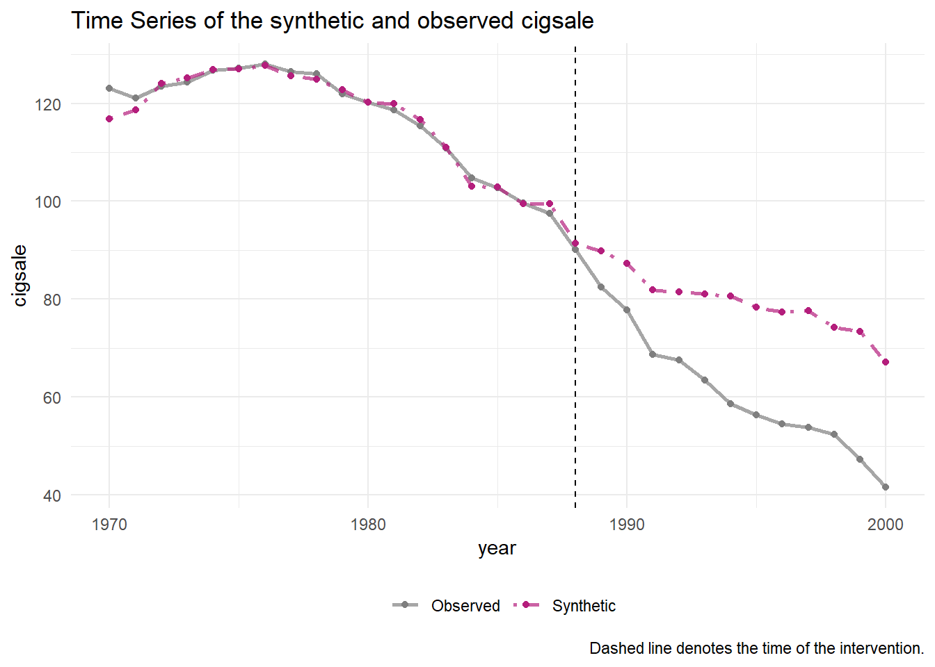
Once the synthetic control is generated, one can easily assess the fit by comparing the trends of the synthetic and observed time series. The idea is that the trends in the pre-intervention period should map closely onto one another.

Code

smoking_out %>% plot_trends()

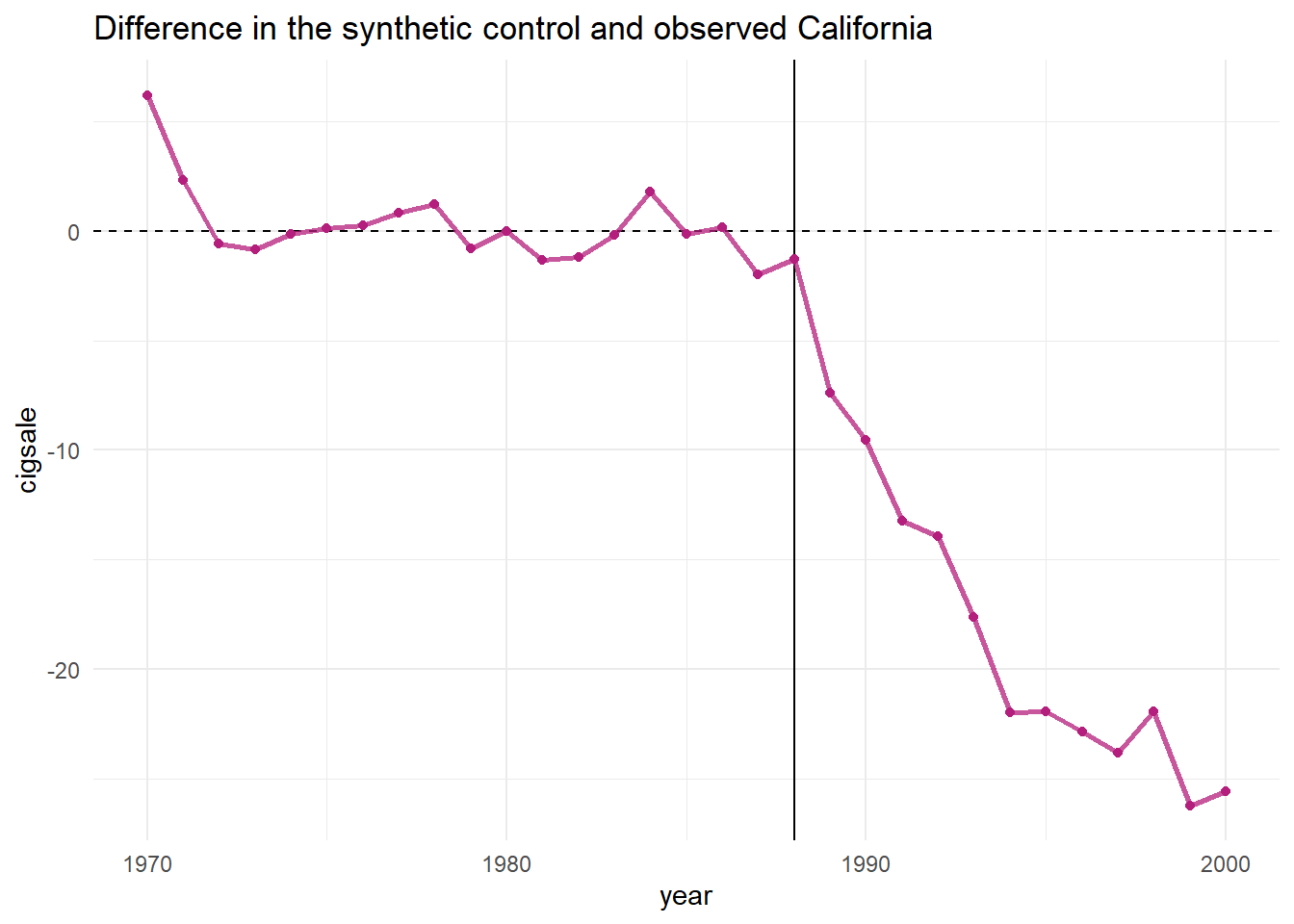
To capture the causal quantity (i.e. the difference between the observed and counterfactual), one can plot the differences using plot_differences()

Code

smoking_out %>% plot_differences()

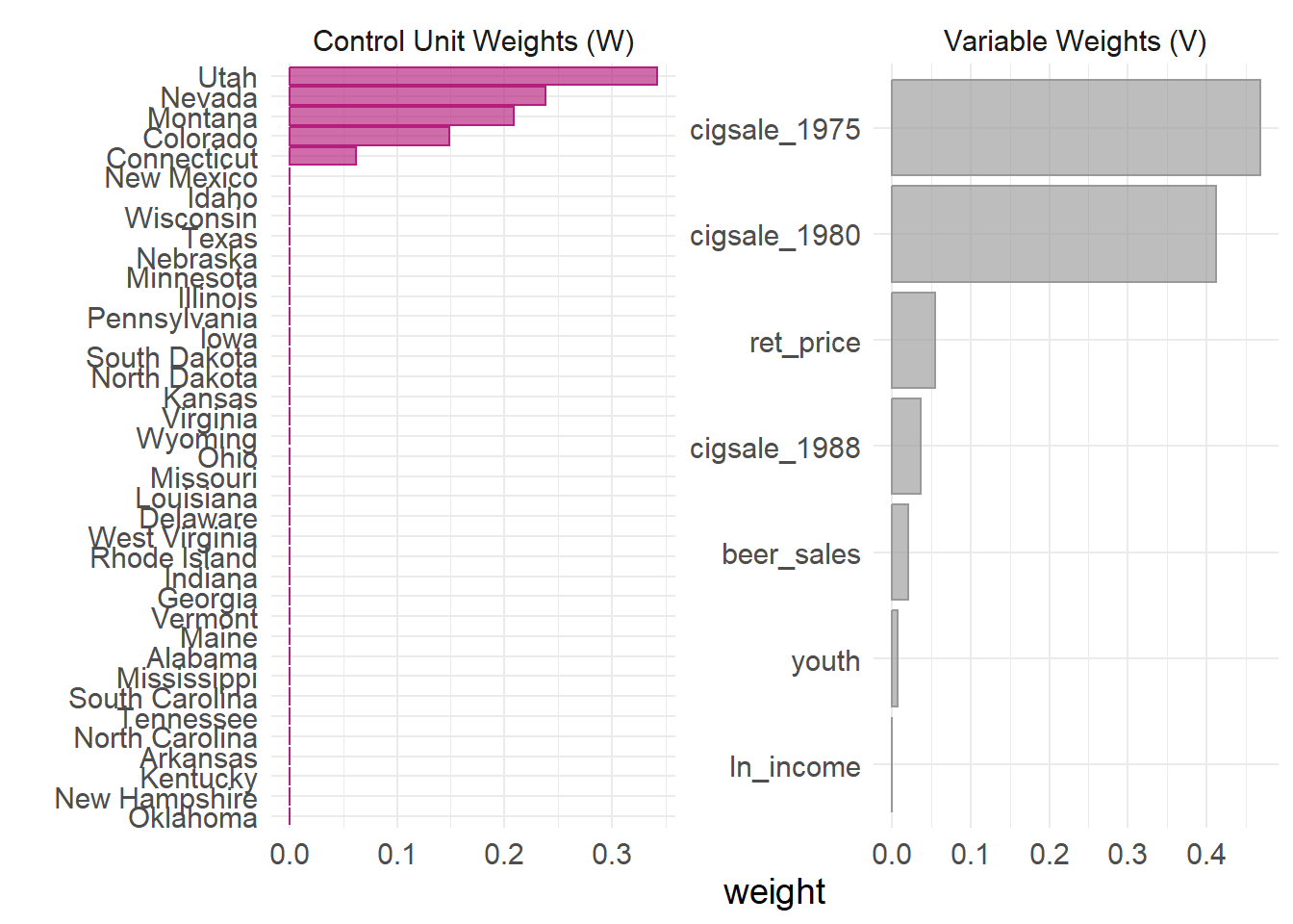
In addition, one can easily examine the weighting of the units and variables in the fit. This allows one to see which cases were used, in part, to generate the synthetic control.

Code

smoking_out %>% plot_weights()

Another useful way of evaluating the synthetic control is to look at how comparable the synthetic control is to the observed covariates of the treated unit.

Code

smoking_out %>% grab_balance_table()

# A tibble: 7 × 4
  variable     California synthetic_California donor_sample
  <chr>             <dbl>                <dbl>        <dbl>
1 ln_income        10.1                  9.85         9.83 
2 ret_price        89.4                 89.4         87.3  
3 youth             0.174                0.174        0.173
4 beer_sales       24.3                 24.2         23.7  
5 cigsale_1975    127.                 127.         137.   
6 cigsale_1980    120.                 120.         138.   
7 cigsale_1988     90.1                 91.4        114.

Inference

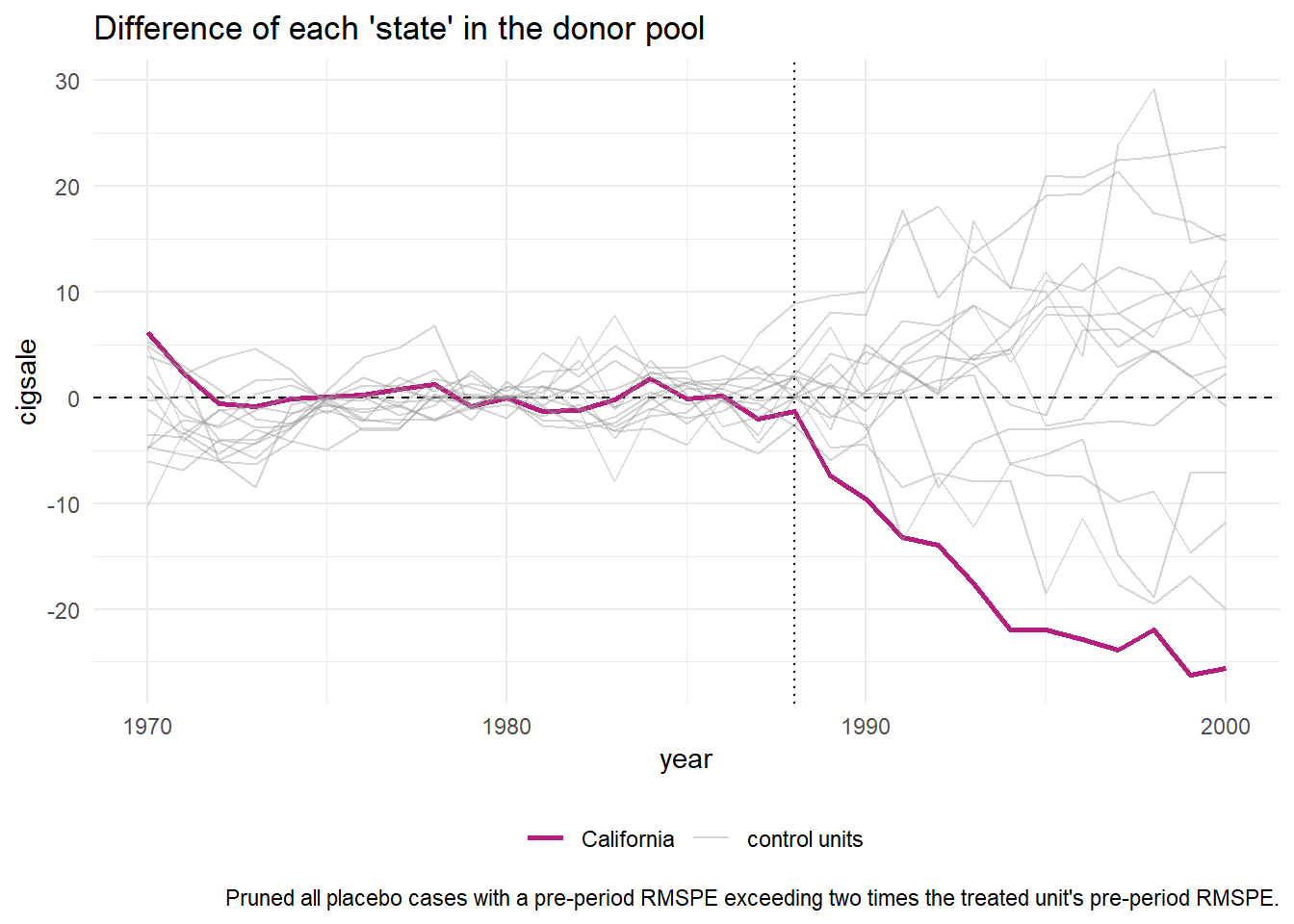
For inference, the method relies on repeating the method for every donor in the donor pool exactly as was done for the treated unit — i.e. generating placebo synthetic controls). By setting generate_placebos = TRUE when initializing the synth pipeline with synthetic_control(), placebo cases are automatically generated when constructing the synthetic control of interest. This makes it easy to explore how unique difference between the observed and synthetic unit is when compared to the placebos.

Code

smoking_out %>% plot_placebos()

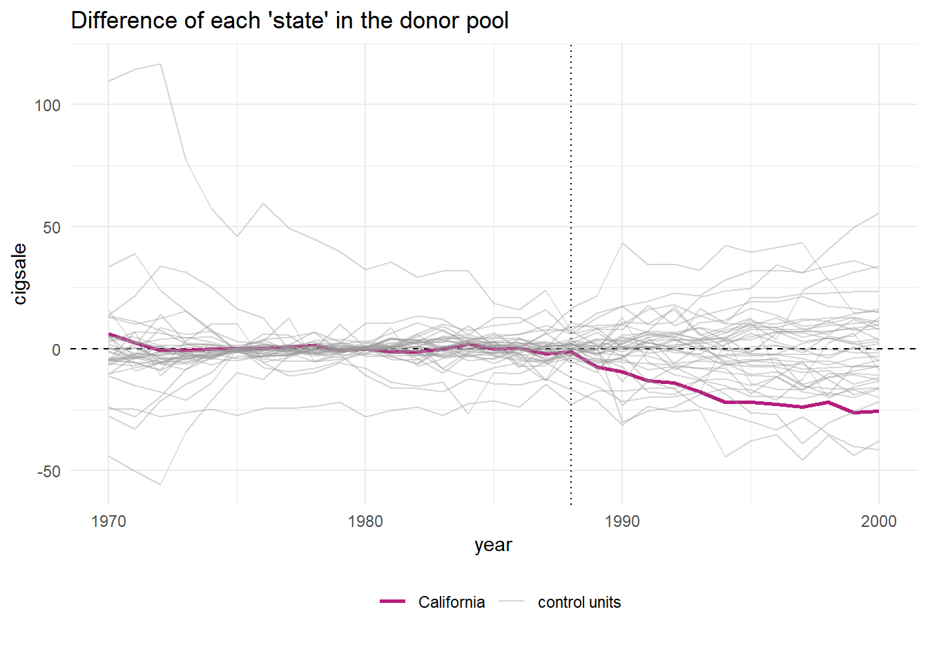
Note that the plot_placebos() function automatically prunes any placebos that poorly fit the data in the pre-intervention period. The reason for doing so is purely visual: those units tend to throw off the scale when plotting the placebos. To prune, the function looks at the pre-intervention period mean squared prediction error (MSPE) (i.e. a metric that reflects how well the synthetic control maps to the observed outcome time series in pre-intervention period). If a placebo control has a MSPE that is two times beyond the target case (e.g. “California”), then it’s dropped. To turn off this behavior, set prune = FALSE.

Code

smoking_out %>% plot_placebos(prune = FALSE)

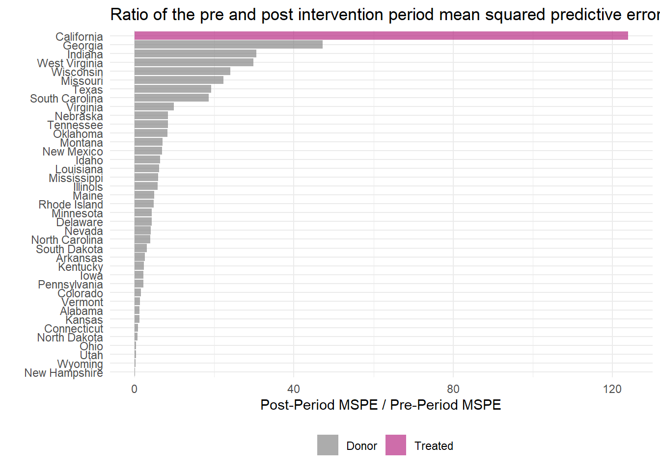
Finally, Adabie et al. 2010 outline a way of constructing Fisher’s Exact P-values by dividing the post-intervention MSPE by the pre-intervention MSPE and then ranking all the cases by this ratio in descending order. A p-value is then constructed by taking the rank/total.1 The idea is that if the synthetic control fits the observed time series well (low MSPE in the pre-period) and diverges in the post-period (high MSPE in the post-period) then there is a meaningful effect due to the intervention. If the intervention had no effect, then the post-period and pre-period should continue to map onto one another fairly well, yielding a ratio close to 1. If the placebo units fit the data similarly, then we can’t reject the hull hypothesis that there is no effect brought about by the intervention.

This ratio can be easily plotted using plot_mspe_ratio(), offering insight into the rarity of the case where the intervention actually occurred.

Code

smoking_out %>% plot_mspe_ratio()

For more specific information, there is a significance table that can be extracted with one of the many grab_ prefix functions.

Code

smoking_out %>% grab_significance()

# A tibble: 39 × 8
   unit_name      type  pre_mspe post_mspe mspe_ratio  rank fishers_exact_pvalue
   <chr>          <chr>    <dbl>     <dbl>      <dbl> <int>                <dbl>
 1 California     Trea…     3.17     392.      124.       1               0.0256
 2 Georgia        Donor     3.79     179.       47.2      2               0.0513
 3 Indiana        Donor    25.2      770.       30.6      3               0.0769
 4 West Virginia  Donor     9.52     284.       29.8      4               0.103 
 5 Wisconsin      Donor    11.1      268.       24.1      5               0.128 
 6 Missouri       Donor     3.03      67.8      22.4      6               0.154 
 7 Texas          Donor    14.4      277.       19.3      7               0.179 
 8 South Carolina Donor    12.6      234.       18.6      8               0.205 
 9 Virginia       Donor     9.81      96.4       9.83     9               0.231 
10 Nebraska       Donor     6.30      52.9       8.40    10               0.256 
# ℹ 29 more rows
# ℹ 1 more variable: z_score <dbl>

References

Treasury, HM. 2020. Magenta Book: Central Government Guidance on Evaluation. HM Treasury. https://www.gov.uk/government/publications/the-magenta-book.